Sleep is key to maintaining a healthy lifestyle. However, it is often overlooked in today’s fast paced world. Sleep efficiency plays a crucial role in insomnia research and it is a commonly used metric to assess sleep quality. By using this sleep efficiency dataset from Morocco, we aim to explore the factors influencing sleep efficiency in a different cultural and geographical context. Understanding the dynamics of sleep patterns and efficiency in Morocco can provide valuable insights into the broader issue of sleep deprivation and its impact on individuals and societies.
While it is true that Singapore is often associated with its competitive nature and struggles with sleep, it is crucial to acknowledge that such issues are not unique to Singapore. Morocco, like many other nations, faces its own unique challenges when it comes to sleep patterns and efficiency. By examining sleep efficiency in Morocco, this project will contribute to the broader conversation about sleep health and its implications, ultimately helping to spur data-driven solutions that can improve sleep patterns and overall well-being on a global scale. Through this project, we aim to predict sleep efficiency based on various factors like age, sleep patterns, and lifestyle choices using a multiple linear regression model.
Dataset
Our dataset is sourced from Kaggle. The variables include ID, Age, Gender, Bedtime, Wakeuptime, Sleep duration, Sleep efficiency, REM sleep percentage, Deep Sleep percentage, Light sleep percentage, Awakenings, Caffeine consumption, Alcohol consumption, Smoking status and Exercise frequency. The understanding and data type of each variable is further explained in our codebook.
Connection to Spark
We initiated a connection to a local Spark cluster and read our Sleep_efficiency.csv file into a Spark DataFrame by employing spark_read_csv(). After which, we saved and read our Parquet file using the spark_write_parquet() and spark_read_parquet() functions. We chose the Apache Parquet format as it allows for efficient data storage and retrieval especially when handling large datasets.
We start off our analysis with data cleaning, first removing rows with nulls, then the ID variable, as they are not needed in our analysis. We then changed smoking_status and gender to binary integer variables instead of categorical variables, changed awakenings to integer, and converted Bedtime and Wakeup_time to hour format. This brings us to 386 observations of 14 variables in our final sleep_clean dataset.
Next, we examined the summary statistics to understand our data further. The average age across the participants is 41 years old, ranging from the youngest at 9 years to the oldest at 69 years old. The average sleep efficiency is 79%, slightly below the National Sleep Foundation (NSF) recommended level at 85%. On average, the participants wake up 1 to 2 times throughout the night. Additionally, exercise frequency is relatively low, typically occurring once or twice a week. On average, participants consume a relatively low amount of caffeine and alcohol, about 23 mg and 1.2 oz respectively. Summary statistics for binary variables are computed to ensure that their minimum and maximum value are 0 and 1 respectively.
In this section, we performed exploratory data analysis to analyse and identify trends amongst our variables.
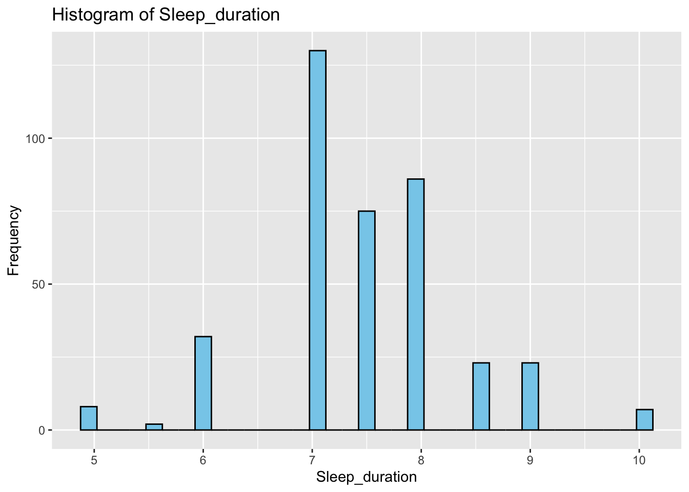
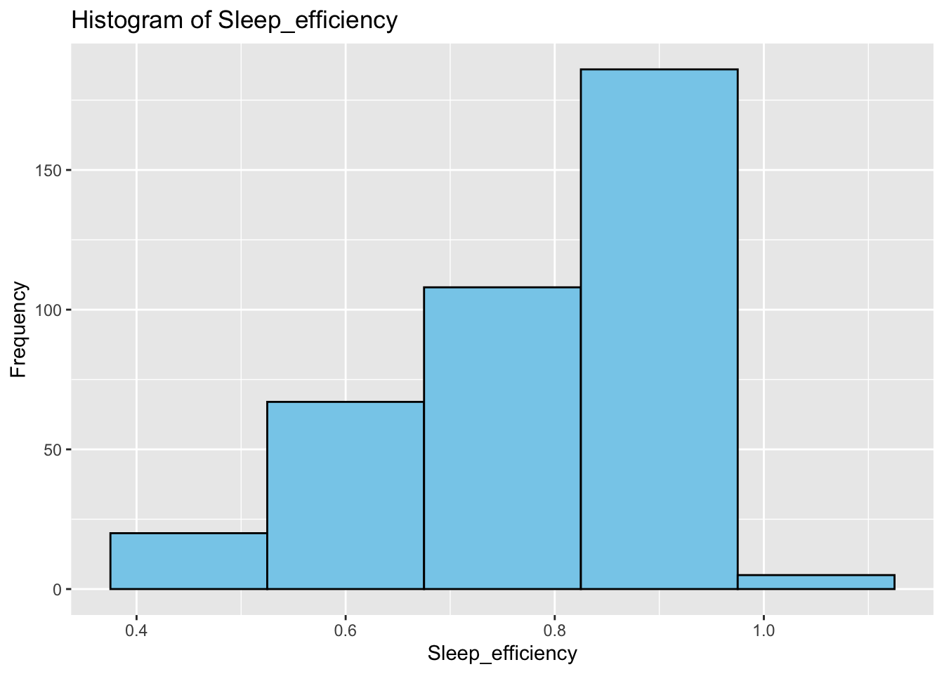
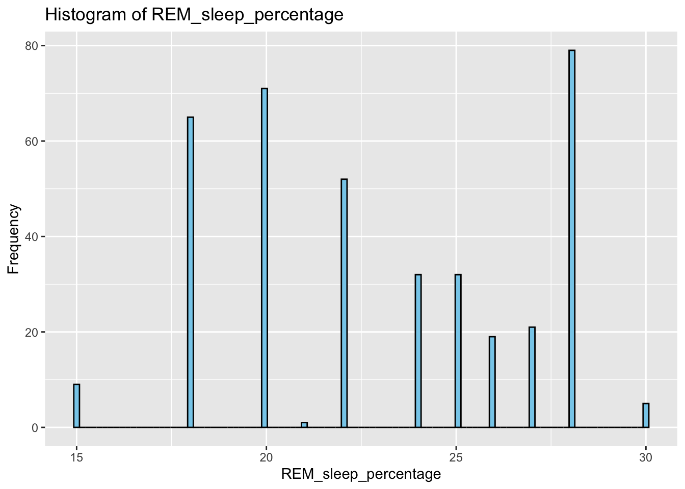
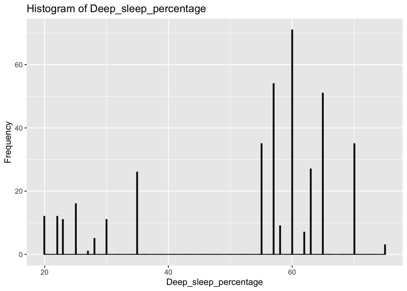
Histogram Frequency plot
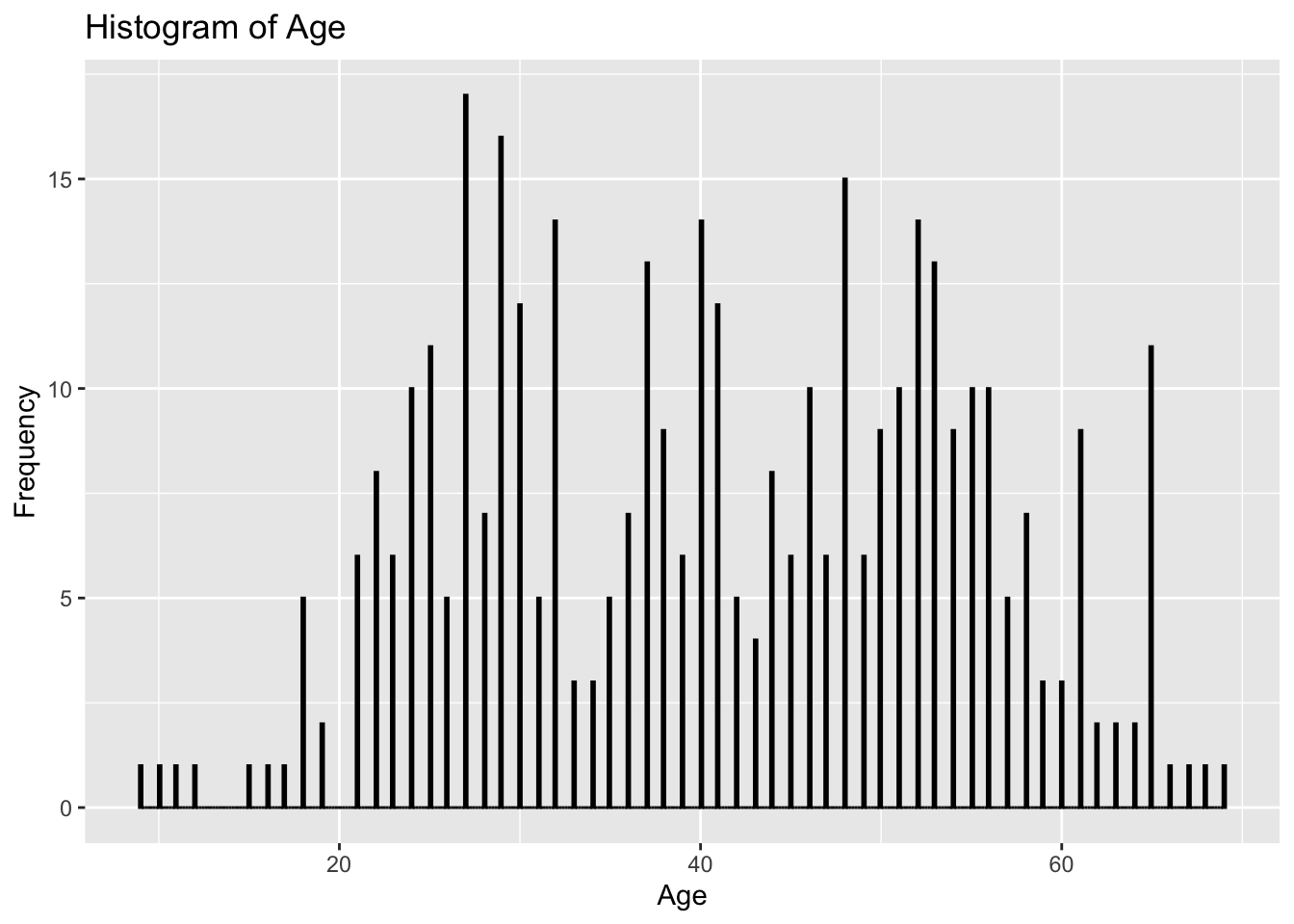
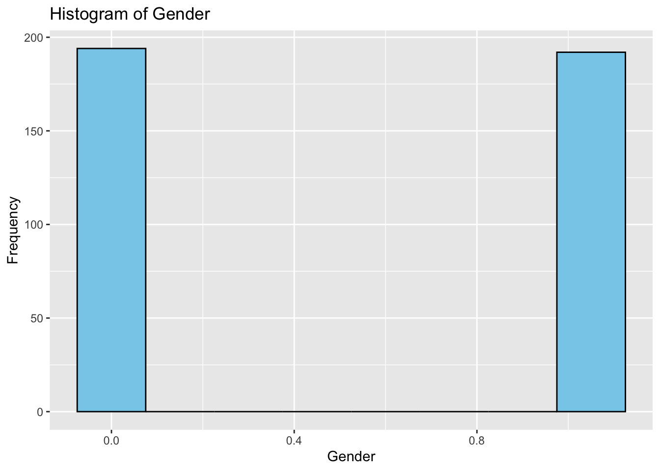
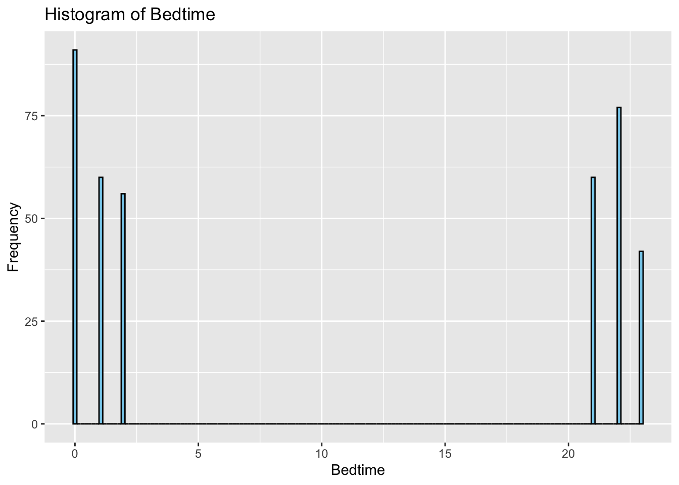
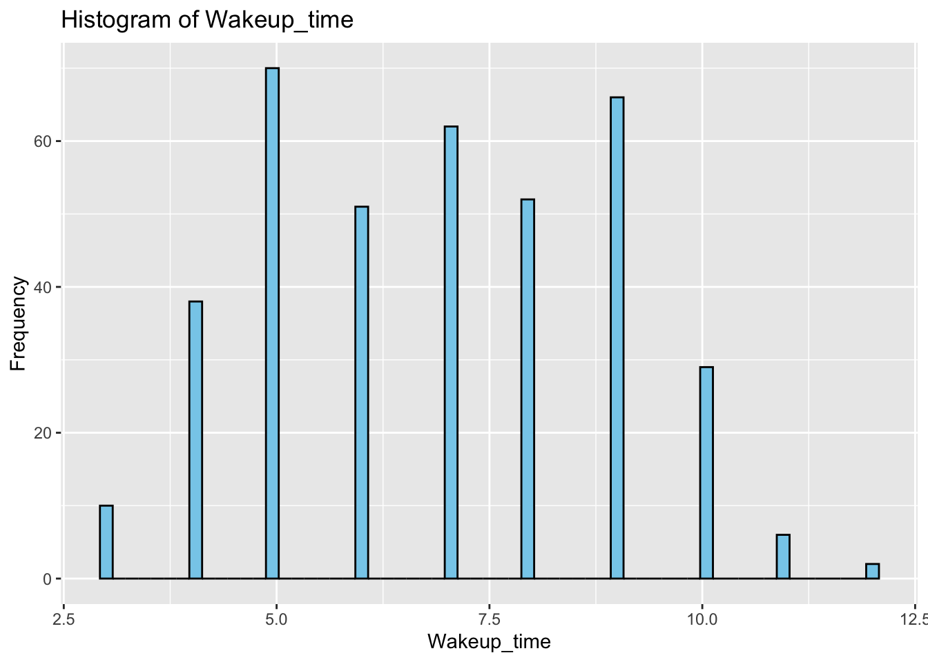
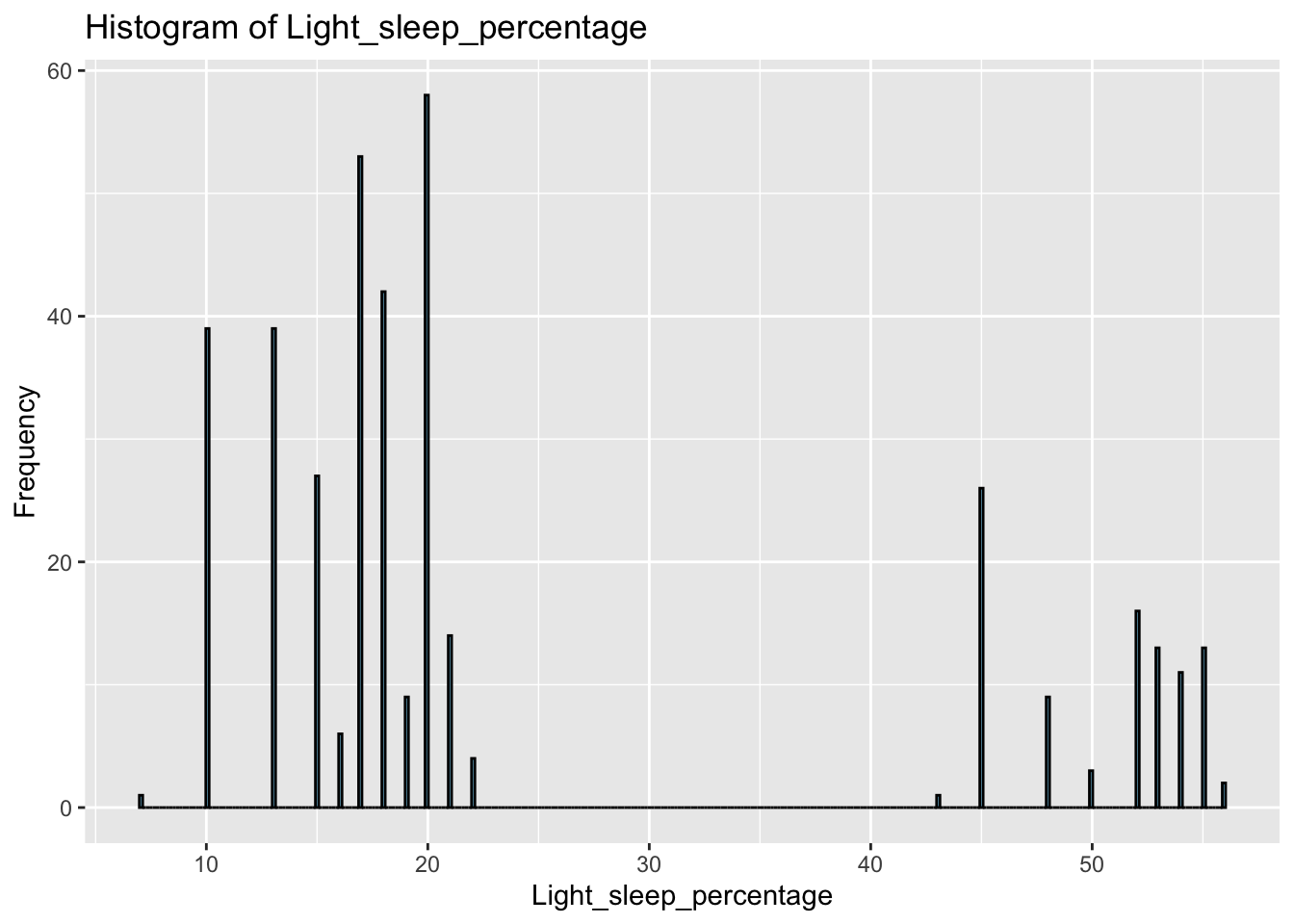
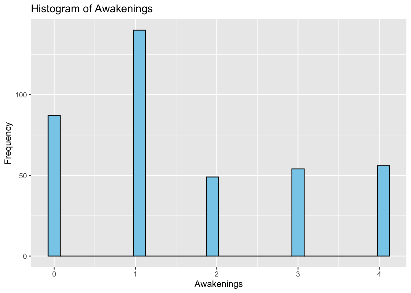
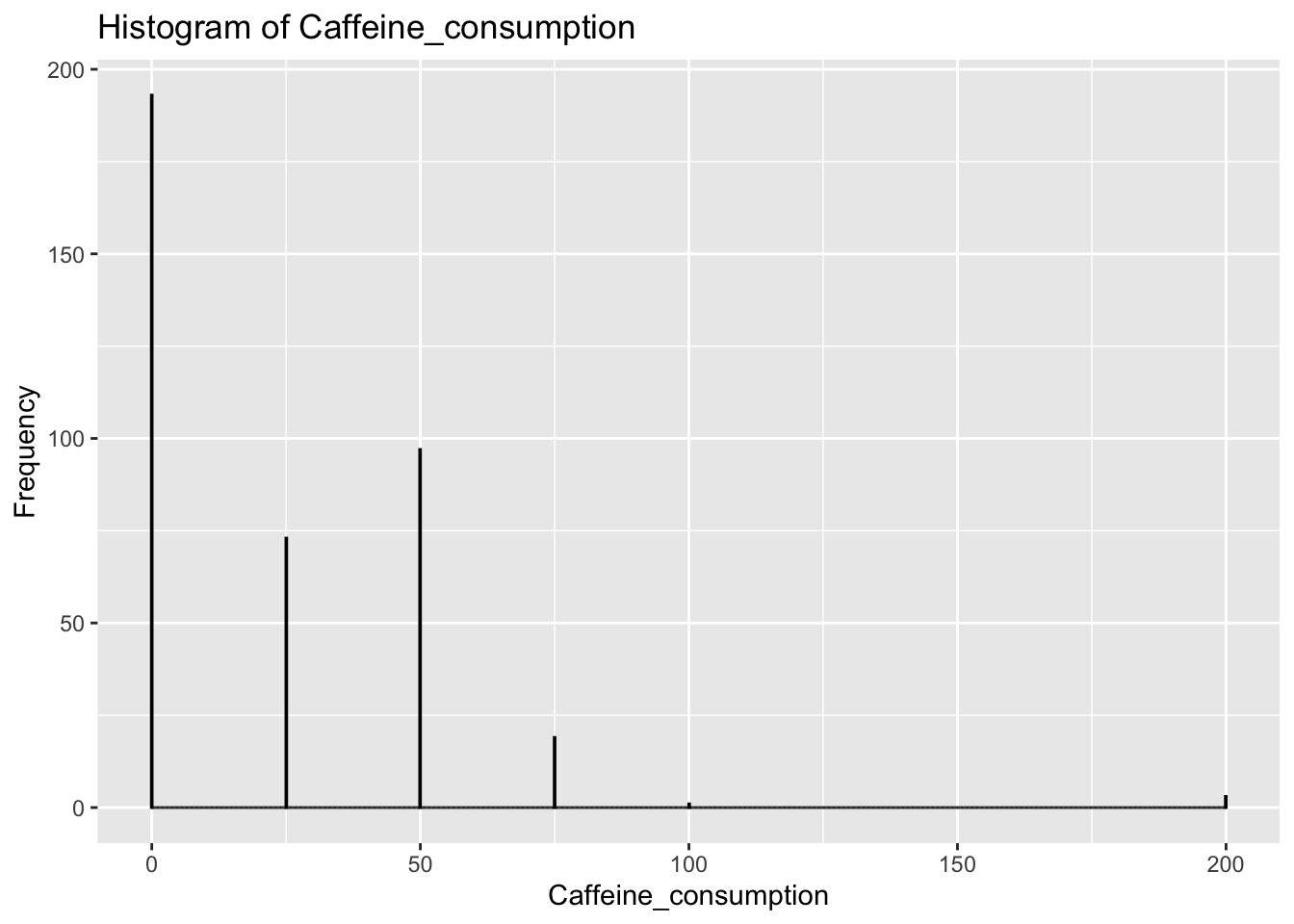
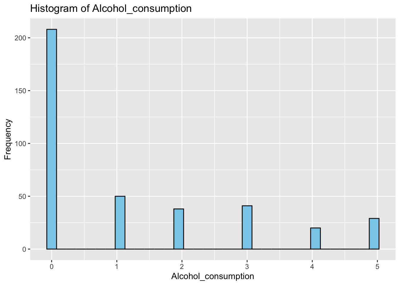
Firstly, we explored 14 variables in the dataset by generating histograms to understand their distribution. From our frequency plots, we can draw the following insights:
Sleep efficiency is relatively high ranging between 0.8 to 0.9.
Age of the participants is concentrated around 25 to 50 years old.
The number of males and females in the dataset appears to be relatively balanced.
Most of the participants experience 7 to 8 hours of sleep per night.
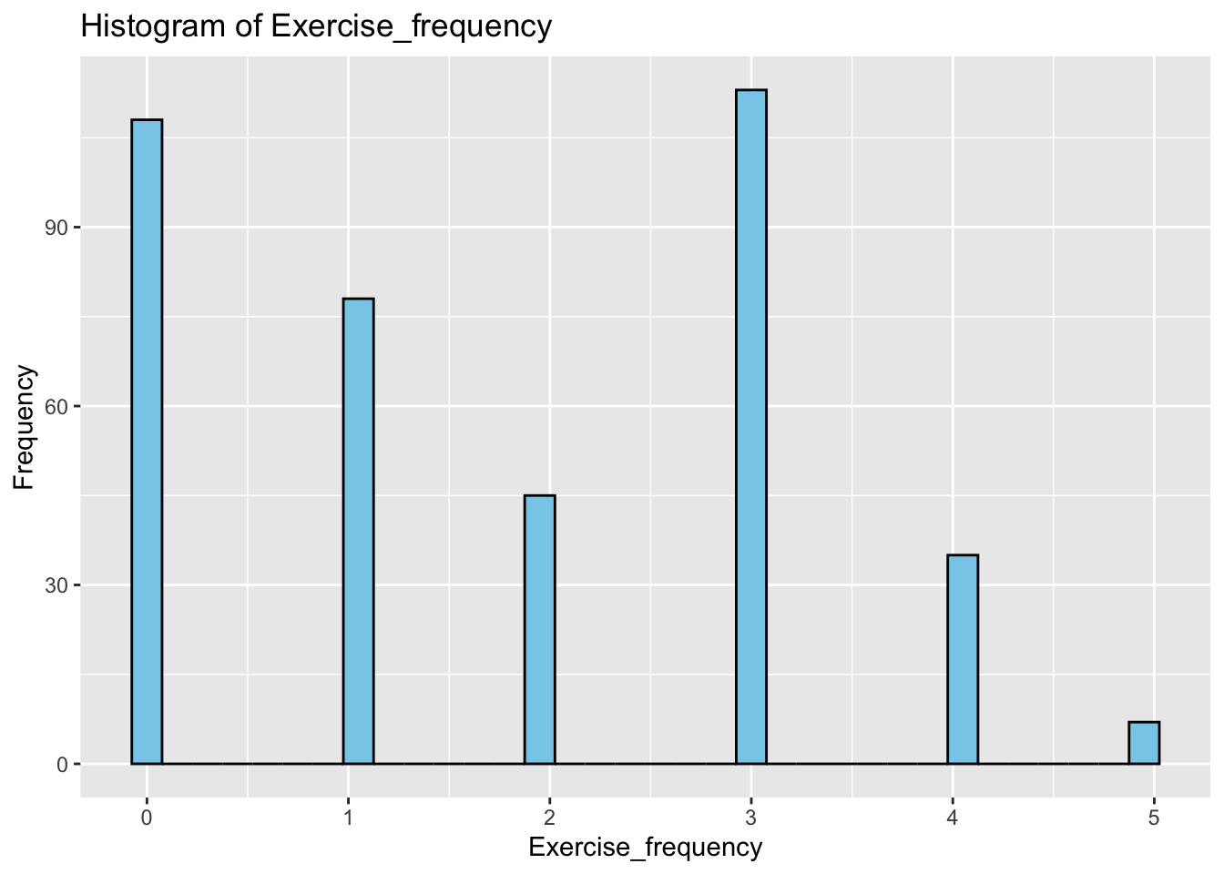
The majority of the participants exercise 0 or 3 times a week.
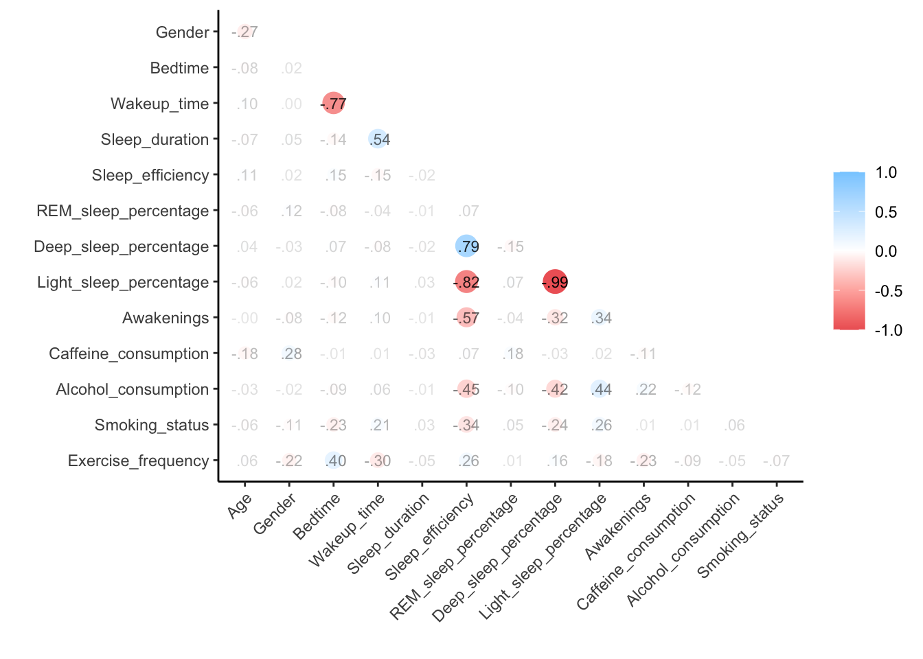
The contrasting patterns of Deep_sleep_percentage and Light_sleep_percentage suggest a potentially high correlation between the two variables.
The majority of the participants woke up 0 or 1 time throughout the night which could explain the relatively high sleep efficiency.
The distribution of Caffeine_consumption is skewed to the right, suggesting that most participants consumed little to no caffeine.
Alcohol consumption is relatively low as the majority appears to consume 0 oz throughout the day.
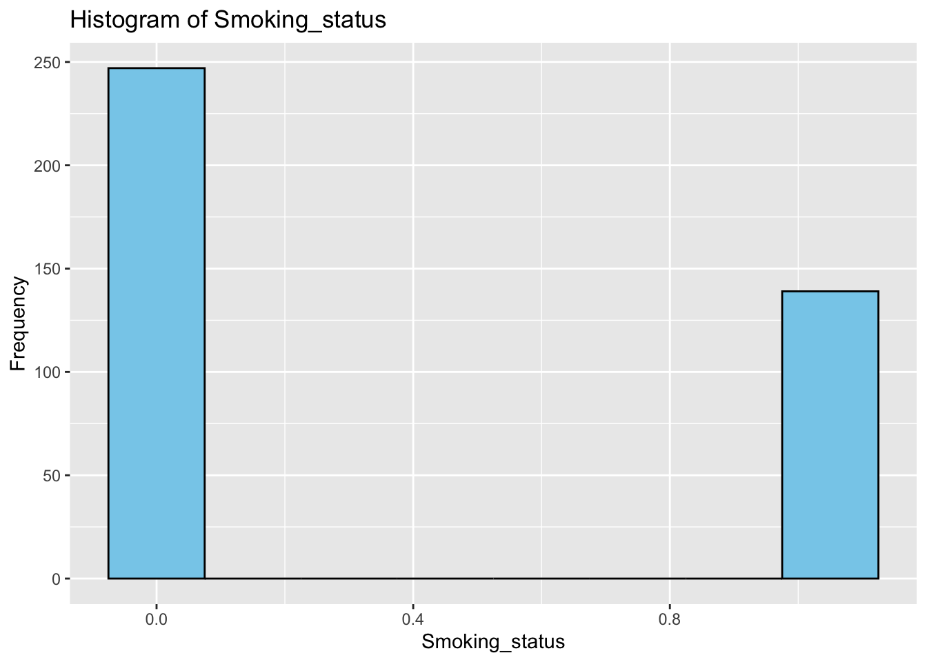
sleep_clean_df <- sleep_clean |>collect() for (col innames(sleep_clean_df)){ graphs <-ggplot(sleep_clean_df, aes_string(x = col)) +geom_histogram(binwidth =0.15, fill ="skyblue", color ="black")+labs(title =paste("Histogram of", col), x = col, y ="Frequency")print(graphs)}
Warning: `aes_string()` was deprecated in ggplot2 3.0.0.
ℹ Please use tidy evaluation idioms with `aes()`.
ℹ See also `vignette("ggplot2-in-packages")` for more information.
Correlation plot
From the correlation plot, Deep_sleep_percentage has the highest correlation with light_sleep_percentage with a correlation coefficient of -0.99. Awakenings has a negative relationship with sleep_efficiency with a correlation coefficient of -0.57, suggesting that as the frequency of awakenings increases, sleep efficiency decreases. Additionally, Deep_sleep_percentage appears to have a strong positive correlation with sleep_efficiency while Light_sleep_percentage has a strong negative correlation with sleep_efficiency.
grouped_sleep1 <- sleep_clean |>mutate(Alcohol_status =ifelse(Alcohol_consumption %in%c(1,2,3,4,5),1,0))|>group_by(Alcohol_status, Smoking_status)|>summarise(n =n())|>group_by(Alcohol_status)|>summarize(count =sum(n), prop =sum(Smoking_status * n) /sum(n))|>#prop of those who smokecollect()
`summarise()` has grouped output by "Alcohol_status". You can override using
the `.groups` argument.
Warning: Missing values are always removed in SQL aggregation functions.
Use `na.rm = TRUE` to silence this warning
This warning is displayed once every 8 hours.
`summarise()` has grouped output by "Alcohol_status". You can override using
the `.groups` argument.
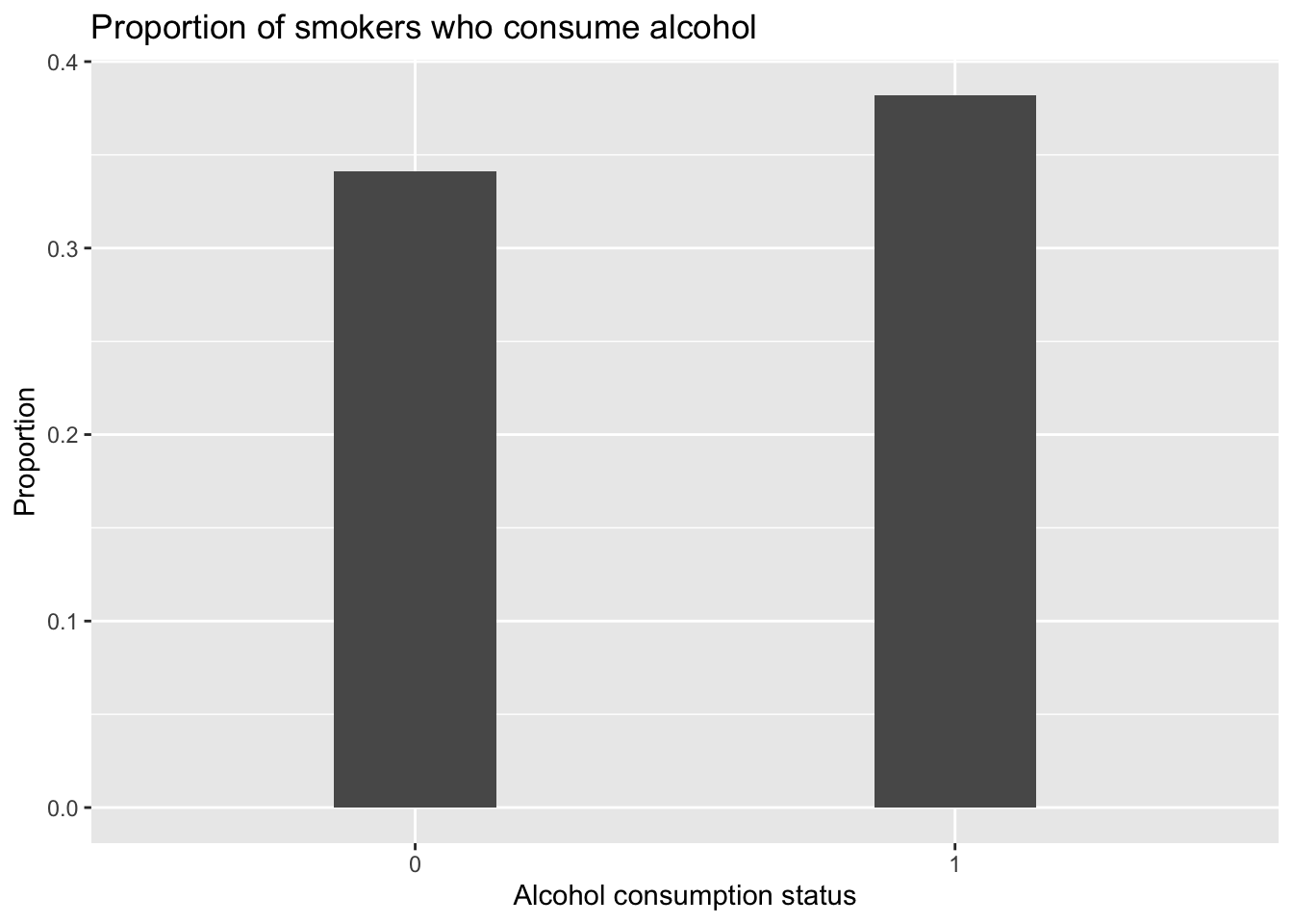
grouped_sleep1 |>mutate(Alcohol_status =as.factor(Alcohol_status))|>ggplot(aes(x = Alcohol_status, y = prop))+geom_col(width =0.3)+labs(title ="Proportion of smokers who consume alcohol")+xlab("Alcohol consumption status")+ylab("Proportion")
Chi-square test for independence for Alcohol consumption and Smoking status
The above plot plot shows that Alcohol_consumption and Smoking_status do not seem to correlate with each other as there is no significant difference between the proportion of smokers who do and do not consume alcohol. Hence, this motivates the use of the chi-square test for independence. Since p-value = 0.5436 > 0.05, we do not reject the null hypothesis at the 5% level of significance and conclude that there is sufficient evidence that smoking status and alcohol consumption are independent.
    Pearson's Chi-squared test with Yates' continuity correction

data:  contingency_matrix
X-squared = 0.36889, df = 1, p-value = 0.5436
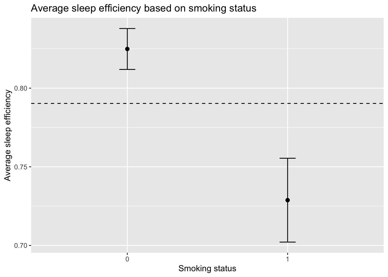
Relationship between Average sleep efficiency and Smoking status
This plot shows the 95% confidence interval of average sleep efficiency for smokers and non-smokers respectively. The dashed line represents the average sleep efficiency (about 0.79) of all the participants regardless of their smoking status. Compared to their smoking counterparts, non-smokers experience a higher sleep efficiency of 0.82 as opposed to 0.72. Furthermore, their sleep efficiency is higher than the overall average. Hence, smoking does have an effect on sleep efficiency.
smoke_prop_data <- sleep_clean |>group_by(Smoking_status) |>summarise(avg_sleep_efficiency =mean(Sleep_efficiency, na.rm =TRUE),sd_sleep_efficiency =sd(Sleep_efficiency, na.rm =TRUE),n =n()) |>mutate(se = sd_sleep_efficiency/sqrt(n)) |>collect()average_sleep_eff_df <- sleep_clean |>summarise(avg_sleep_efficiency =mean(Sleep_efficiency))|>collect()average_sleep_eff_vec <- average_sleep_eff_df$avg_sleep_efficiency#plotting relationship between smoking status and sleep efficiencysmoke_prop_data |>mutate(Smoking_status =as.factor(Smoking_status))|>ggplot(aes(x = Smoking_status, y = avg_sleep_efficiency))+geom_point(size =2)+geom_errorbar(aes(ymin = avg_sleep_efficiency -1.96*se,ymax = avg_sleep_efficiency +1.96*se),width =0.1) +geom_hline(yintercept = average_sleep_eff_vec, linetype ="dashed")+labs(title ="Average sleep efficiency based on smoking status")+ylab("Average sleep efficiency")+xlab("Smoking status")
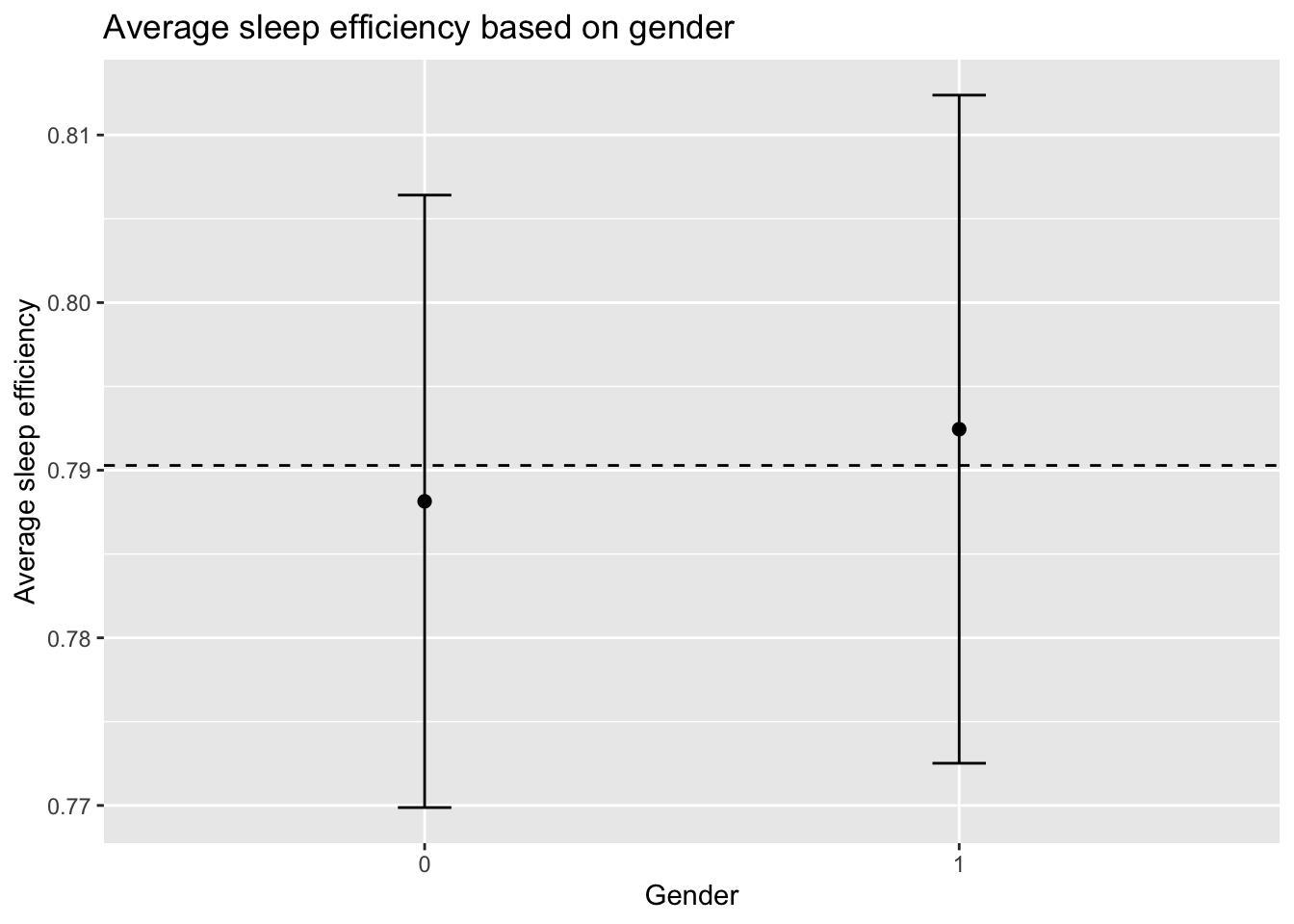
Relationship between Average sleep efficiency and Gender
Similarly, the interval plot shows the 95% confidence interval for average sleep efficiency of both male and female. Dashed line represents the average sleep efficiency regardless of gender. Females experience a slightly higher sleep quality as compared to males, and the overall average. However, there is no significant difference in average sleep efficiency between the two groups. Hence gender does not affect sleep efficiency.
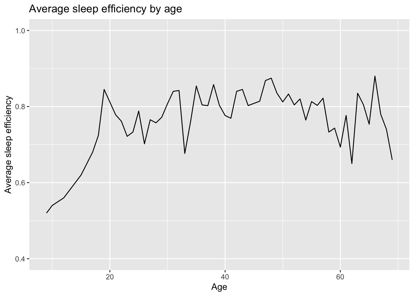
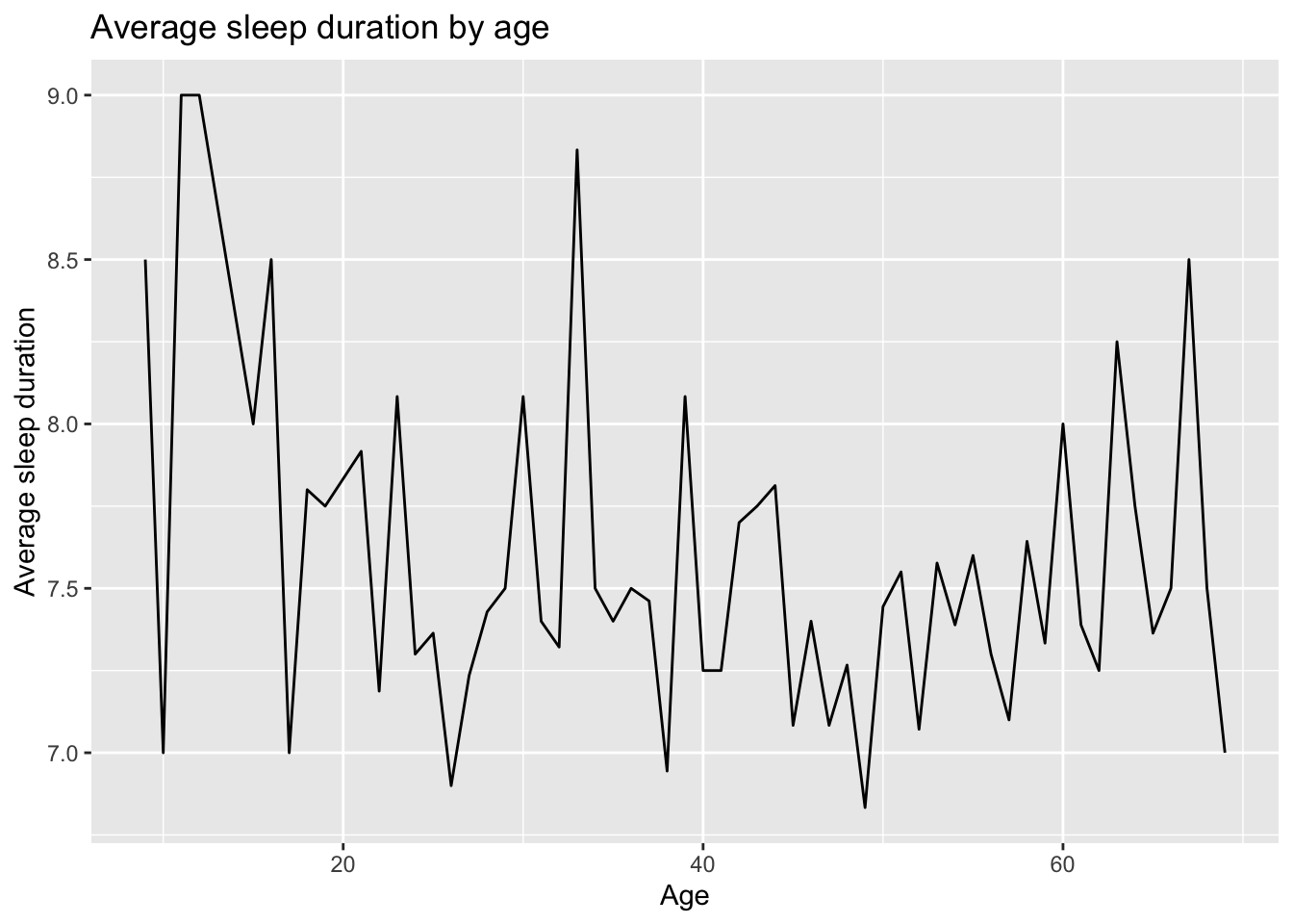
Relationship between Age, Sleep duration and Sleep efficiency
From the line graph, participants in their early 30s experienced a significant drop in sleep efficiency, despite having the second longest sleeping duration across all age groups. This suggests that they might have trouble falling asleep which implies that they spend more time awake while in bed. Therefore, a longer sleep duration does not necessarily lead to a higher sleep efficiency.
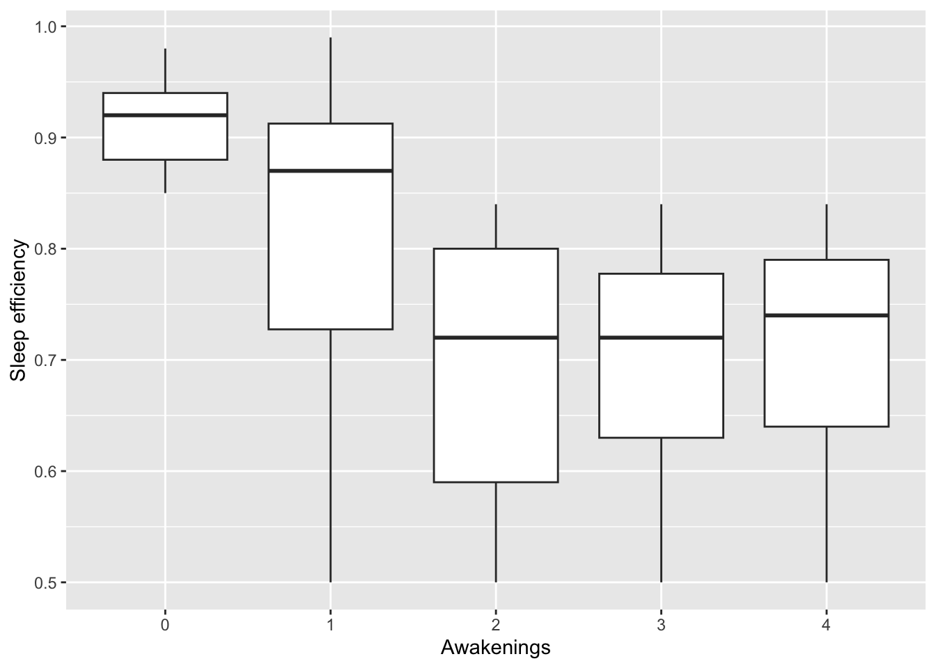
Relationship between Sleep efficiency and Awakenings
From the box plot, sleep efficiency is the highest when participants did not wake up during the night. The average sleep efficiency is 0.92, surpassing the NSF’s recommended value of 0.85. Sleep efficiency is approximately 0.7 for individuals who woke up 2, 3 or 4 times during the night. This indicates that Awakenings might be useful to predict sleep efficiency for individuals experiencing less disrupted sleep.
sleep_clean |>ggplot(aes(x =as.factor(Awakenings), y = Sleep_efficiency)) +geom_boxplot() +xlab("Awakenings") +ylab("Sleep efficiency")
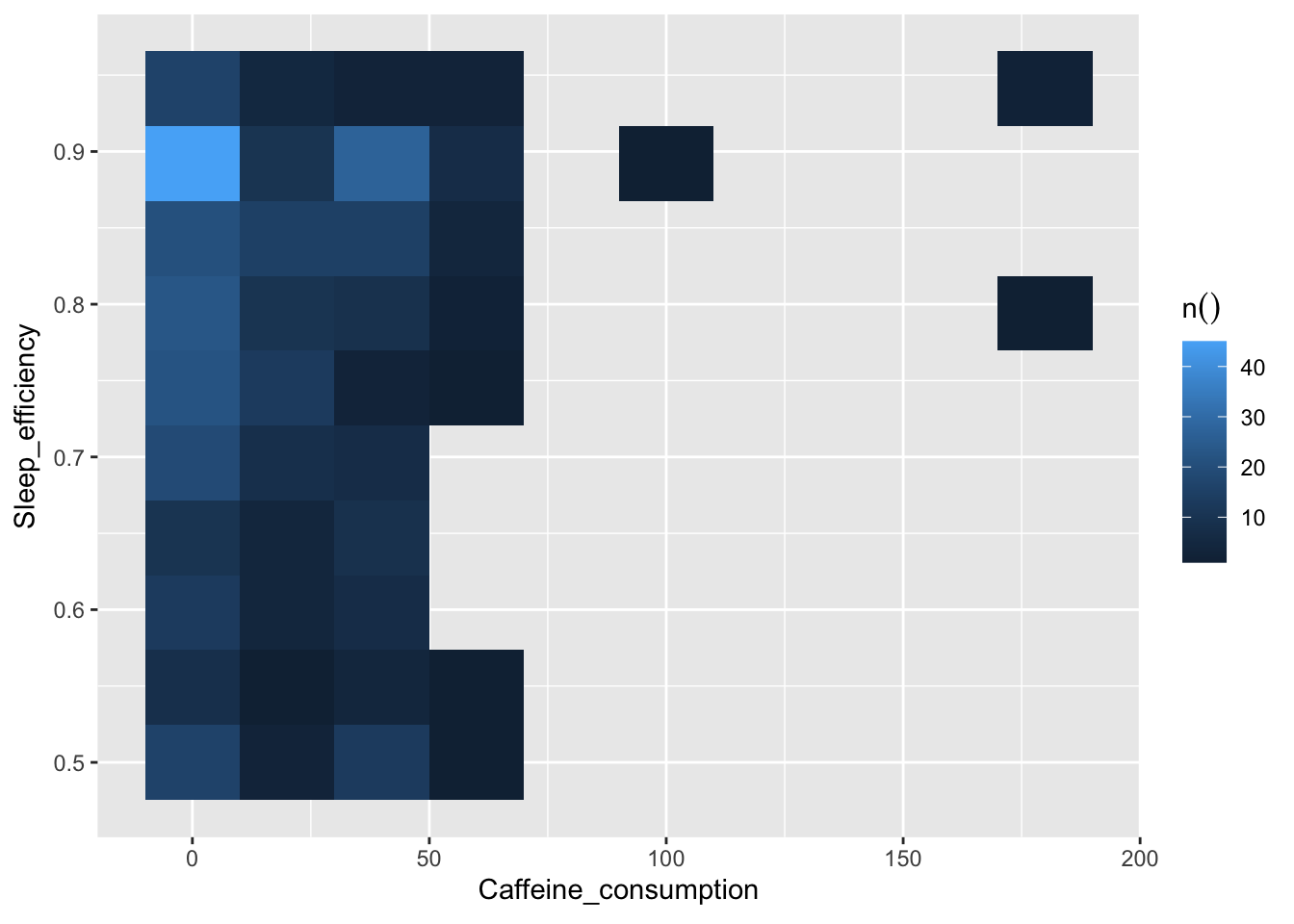
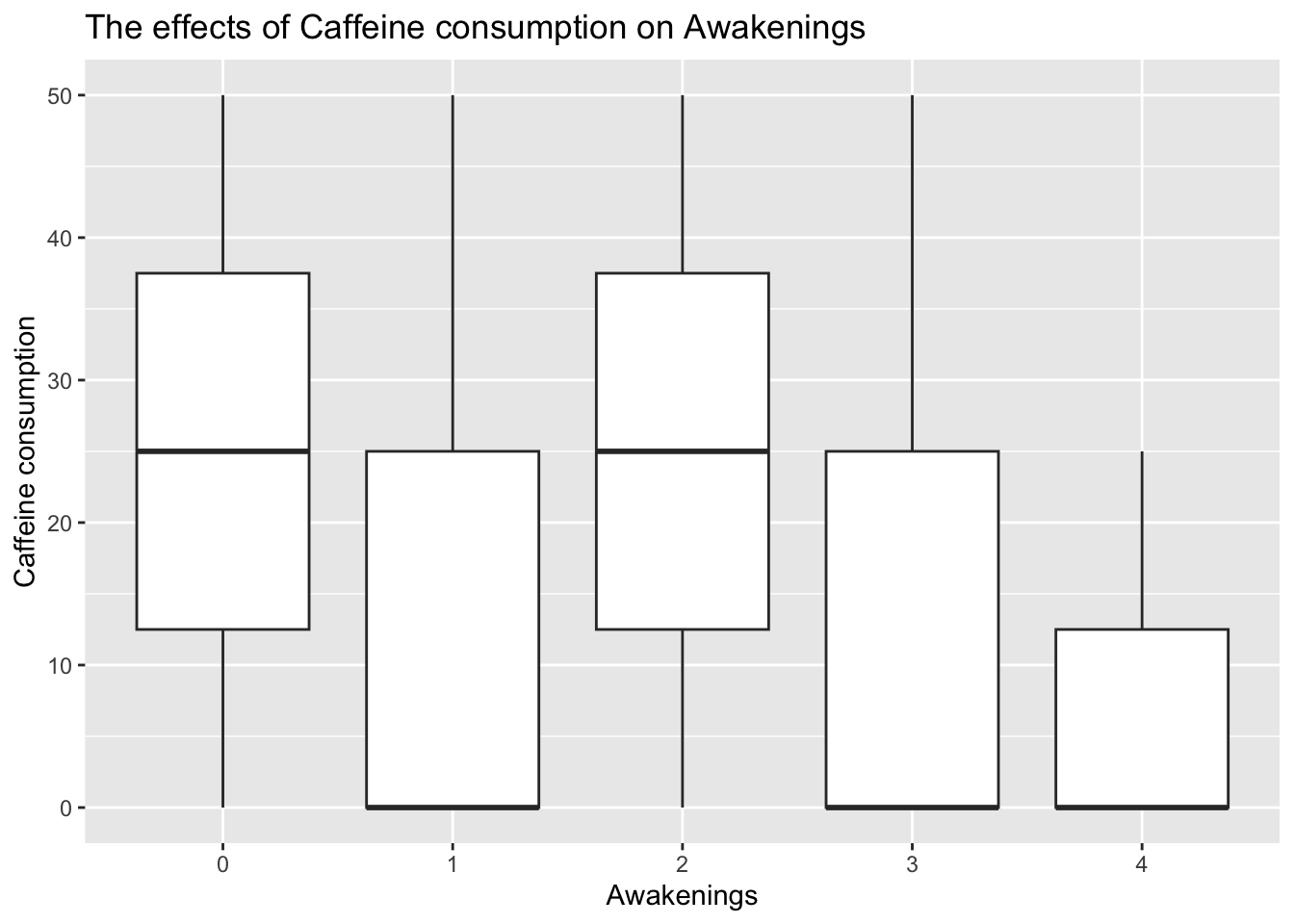
Relationship between Sleep efficiency and Caffeine consumption
One can experience varying levels of sleep efficiency even when 0 mg of caffeine is consumed. As shown in the raster plot, there are outliers that show that sleep efficiency can be as high as 0.9 even when a high dose of caffeine is consumed. Hence, caffeine consumption might not be a significant variable. Moreover, the box plot shows that caffeine consumption does not seem to affect Awakenings as well. This suggests that caffeine might not necessarily affect sleep efficiency in this context. Nonetheless, if a larger sample size or additional information about the timing of caffeine consumption were available, it might provide a clearer understanding of this relationship.
sleep_clean |>dbplot_raster(x = Caffeine_consumption, y = Sleep_efficiency, fill =n(), resolution =10)
grouped_sleep4 <- sleep_clean |>group_by(Awakenings)|>summarise(Caffeine_consumption_percentile =percentile(Caffeine_consumption, array(0.25,0.5,0.75)))|>mutate(Caffeine_consumption_percentile =explode(Caffeine_consumption_percentile))|>collect()grouped_sleep4 |>mutate(Awakenings =as.factor(Awakenings))|>ggplot(aes(x = Awakenings, y = Caffeine_consumption_percentile))+geom_boxplot()+labs(title ="The effects of Caffeine consumption on Awakenings")+ylab("Caffeine consumption")+xlab("Awakenings")
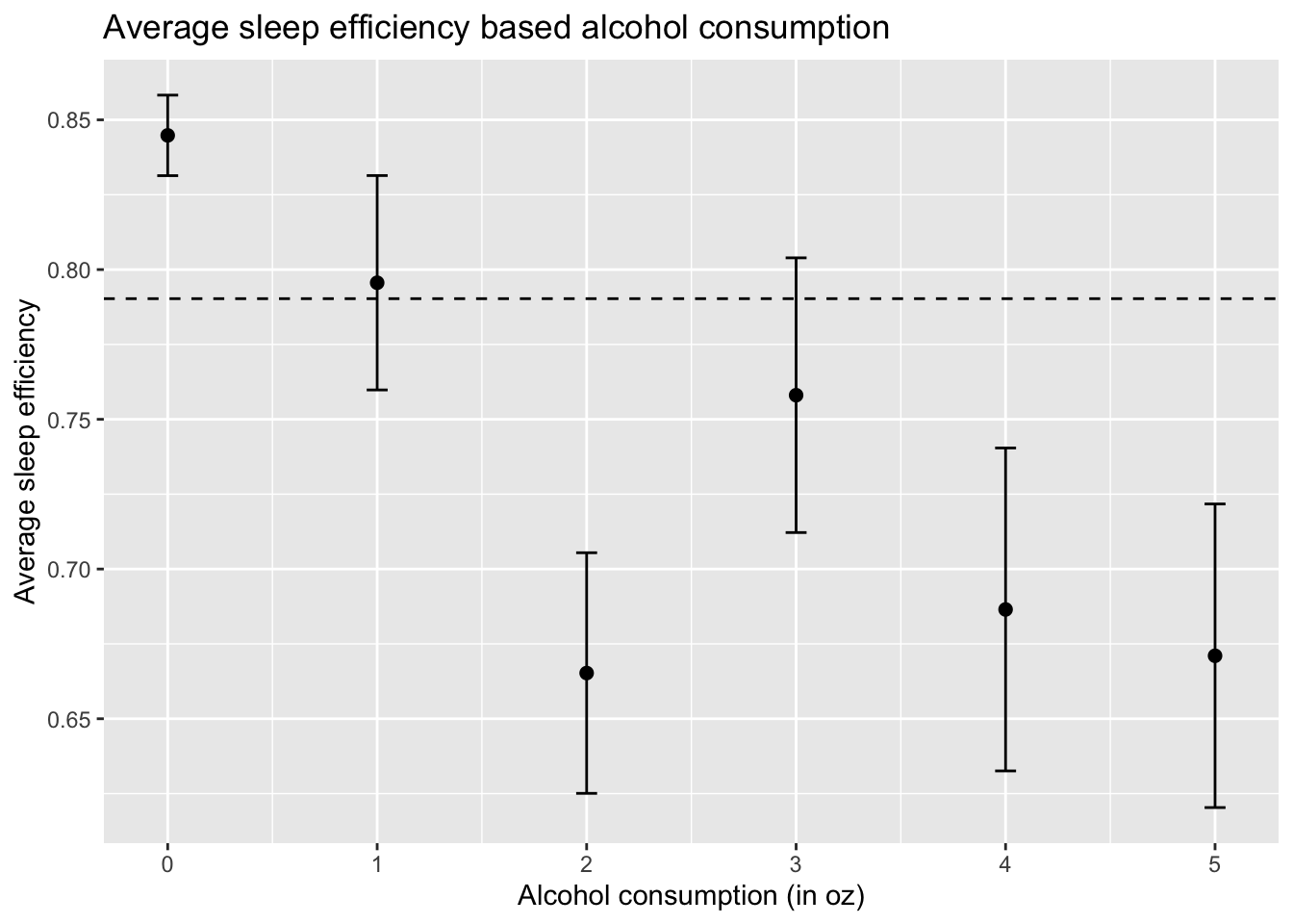
Relationship between Sleep efficiency and Alcohol consumption
The interval plot shows the 95% confidence interval for average sleep efficiency based on the alcohol consumption level. In general, an increase in alcohol consumption generally results in decreased sleep efficiency.
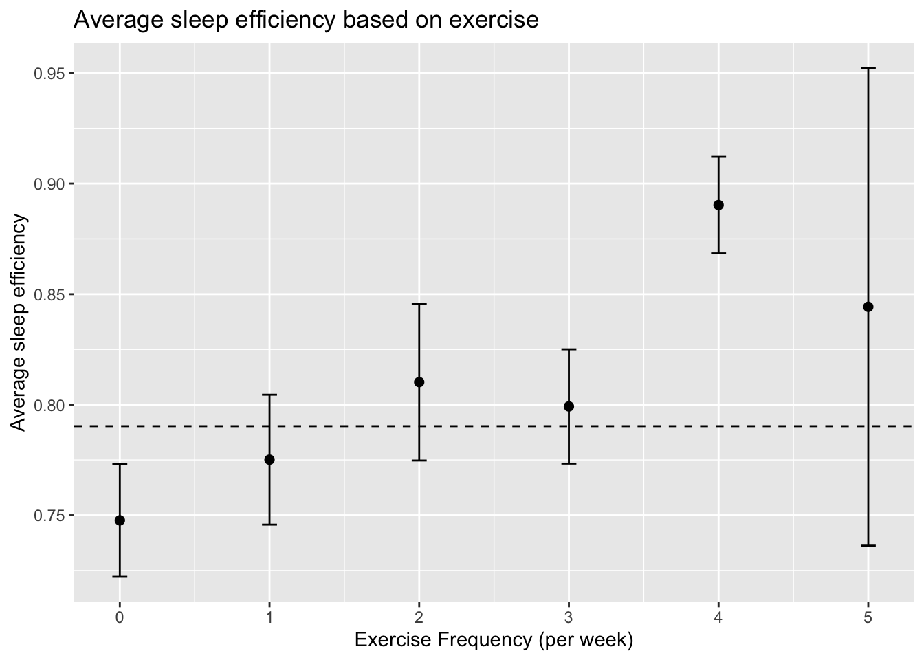
Relationship between Sleep efficiency and Exercise frequency
The interval plot shows the 95% confidence interval for average sleep efficiency based on the exercise frequency. We can observe that exercising generally improves sleep efficiency, but the benefits of exercising more than once a week is hard to discern because the confidence intervals for frequencies 1 to 5 all overlap the average sleep efficiency level.
exercise_prop_data <- sleep_clean |>group_by(Exercise_frequency) |>summarise(avg_sleep_efficiency =mean(Sleep_efficiency),sd_sleep_efficiency =sd(Sleep_efficiency),n =n())|>mutate(se = sd_sleep_efficiency/sqrt(n)) |>arrange(Exercise_frequency) |>collect()#plotting relationship between exercise and sleep efficiencyexercise_prop_data |>ggplot(aes(x = Exercise_frequency, y = avg_sleep_efficiency))+geom_point(size =2)+geom_errorbar(aes(ymin = avg_sleep_efficiency -1.96*se,ymax = avg_sleep_efficiency +1.96*se),width =0.1) +geom_hline(yintercept = average_sleep_eff_vec, linetype ="dashed")+labs(title ="Average sleep efficiency based on exercise")+ylab("Average sleep efficiency")+xlab("Exercise Frequency (per week)")
Relationship between Bedtime and Sleep efficiency
The plot shows the average sleep efficiency across various bedtimes. The size of the points represents the number of individuals who slept at each time. Majority of the participants tend to sleep at either 10pm or 12am. Sleep efficiency is the highest when individuals go to bed at 10pm and starts to drop thereafter.
Upon closer examination, the plot shows the scatter plots after filtering for cases where sleep efficiency was above average level of 0.79, and sleep duration was at least 7 hours.
grouped_sleep5 <- sleep_clean |>group_by(Bedtime)|>summarise(n =n(), ave_sleep =mean(Sleep_efficiency))|>arrange(desc(ave_sleep))|>collect()bedtime_plot <- grouped_sleep5 |>mutate(Bedtime =as.factor(Bedtime)) |>ggplot(aes(x=Bedtime, y=ave_sleep))+geom_point(aes(size = n))+labs(title ="The effects of Bedtime on Sleep efficiency")+ylab("Average sleep efficiency")+xlab("Bedtime in 24 Hours")+theme_minimal()ggplotly(bedtime_plot)
`summarise()` has grouped output by "Bedtime". You can override using the
`.groups` argument.
bedtime_plot <- grouped_sleep6 |>mutate(Bedtime =as.factor(Bedtime)) |>ggplot(aes(x=Bedtime, y=ave_sleep))+geom_point(aes(size = n))+geom_point(aes(colour= Sleep_duration))+labs(title ="The effects of Bedtime on Sleep efficiency")+ylab("Average sleep efficiency")+xlab("Bedtime in 24 Hours")+theme_minimal()ggplotly(bedtime_plot)
3. Data Modelling in Spark
In this section, we aim to use machine learning models to conduct predictive modelling. We used multiple linear regression to predict sleep efficiency. The first model includes all the variables except for Bedtime and Wakeup_time to avoid perfect collinearity problem as they have a linear relationship with Sleep_duration. In the second model, Deep_sleep_percentage is removed to avoid multicollinearity as it is highly correlated with Light_sleep_percentage. Additionally, our visualisations have shown that Gender, Sleep_duration and Caffeine_consumption does not affect sleep efficiency. Moreover, given that their p-value in the first regression is more than 0.05, it suggests that they are not statistically significant. Hence they are excluded from our second model. Lastly, the third model is the same as the second model but includes Caffeine_consumption.
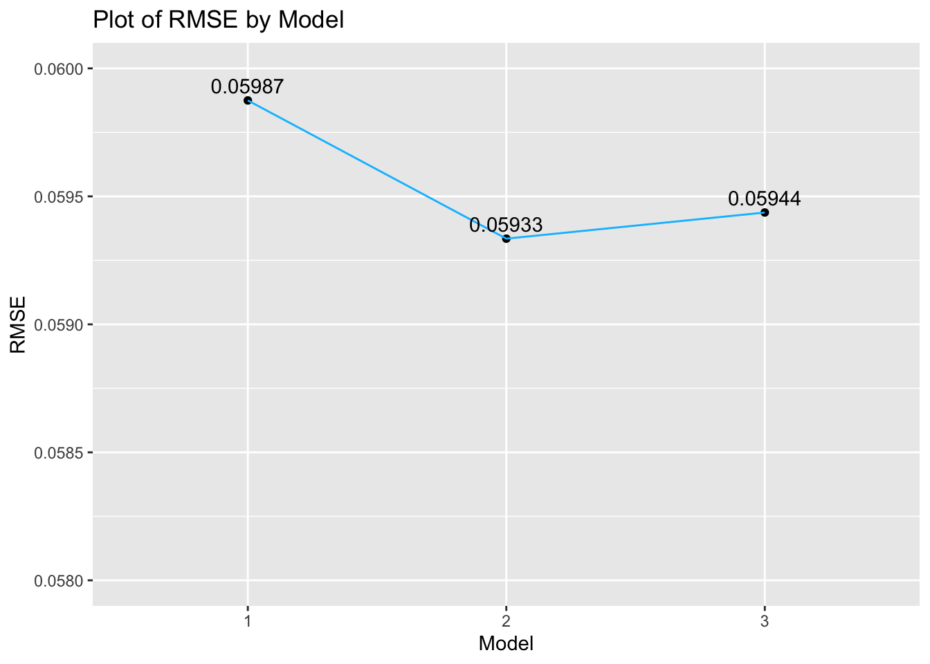
To find the best model, we employed a 10-fold cross-validation by using ml_cross_validator() to compare their Root Mean Squared Error (RMSE). The parameters of elastic_net_param and reg_param are set to zero to perform the least squares. (Ridge regression without penalty). From the RMSE plot, it shows that the RMSE for Model 2 is the lowest (0.05933). Nonetheless, Model 3 with added the variable: caffeine_consumption, is still chosen to be the best model to predict sleep efficiency. As this plot employs ggplot(), it is important to note that the axes are automatically scaled and the difference in RMSE between the models differ slightly in absolute terms despite the huge drop reflected in the line graph.
Despite the slight increase in Model 3’s RMSE, we still chose to include caffeine_consumption in our final model. The prevalence of tea drinking as part of Moroccan culture explains the relatively low amount of caffeine consumed (about 23 mg) per person. However, it is still an important variable to predict sleep efficiency for individuals outside Morocco, where higher levels of caffeine consumption is more prevalent.
Firstly, a pipeline of 6 stages is created. All numerical variables in Model 3 are standardised with mean equals to 0 and standard deviation equals to 1. Next, Smoking_status is indexed and encoded. Finally, all variables go through the ml_linear_regression() stage. The pipeline was created using a for-loop, as we have treated our dataset as if it were big data with more variables. In reality, there could be more categorical variables in the regression to be indexed and encoded. Therefore, this is a more efficient approach and improves the readability of the pipeline.
Then, cross validation with different combinations of elastic_net_param from values 0 to 1 is employed. The initial value for reg_param starts from 0.001 instead of 0 because it gives us a model with a lower RMSE. Finally, the improved model has a slightly lower RMSE of 0.05939 with the following hyperparameters – elastic_net_param_1 = 0 and reg_param_1 = 0.00289.
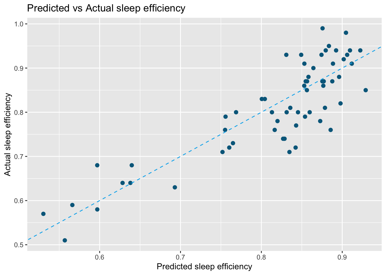
Predict sleep efficiency on the test set using the best model after hyperparameter tuning. This plot shows the actual against predicted sleep efficiency. The model performs relatively well in predicting individuals with sleep efficiency between 0.85 to 0.90.
predictions |>ggplot(aes(x = prediction, y = Sleep_efficiency)) +geom_point(color ="deepskyblue4", size =2) +geom_abline(color ="deepskyblue2", linetype ="dashed") +labs(x ="Predicted sleep efficiency",y ="Actual sleep efficiency",title ="Predicted vs Actual sleep efficiency" )